Lessons I Learned From Info About How To Draw Chart Excel
How To Make A Graph In Excel: Step By Detailed Tutorial
How To Create A Chart Or Graph In Excel?
How To Make A Bar Chart In Microsoft Excel
How To Create Charts In Excel (in Easy Steps)
Excel 2013: Charts
How To Make A Bar Graph In Excel

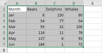
Set up the data first.
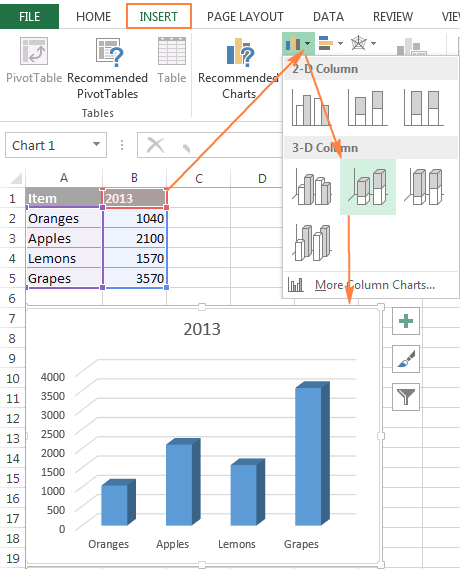
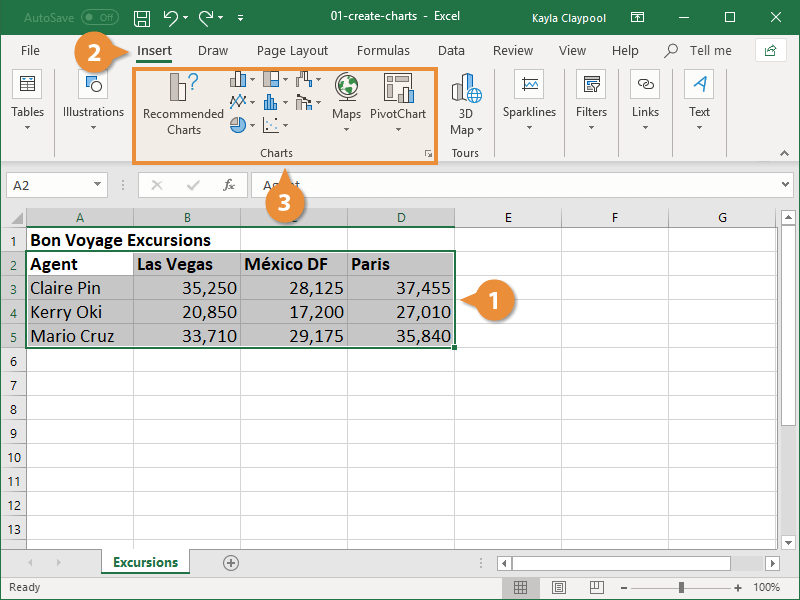
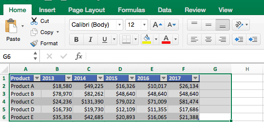
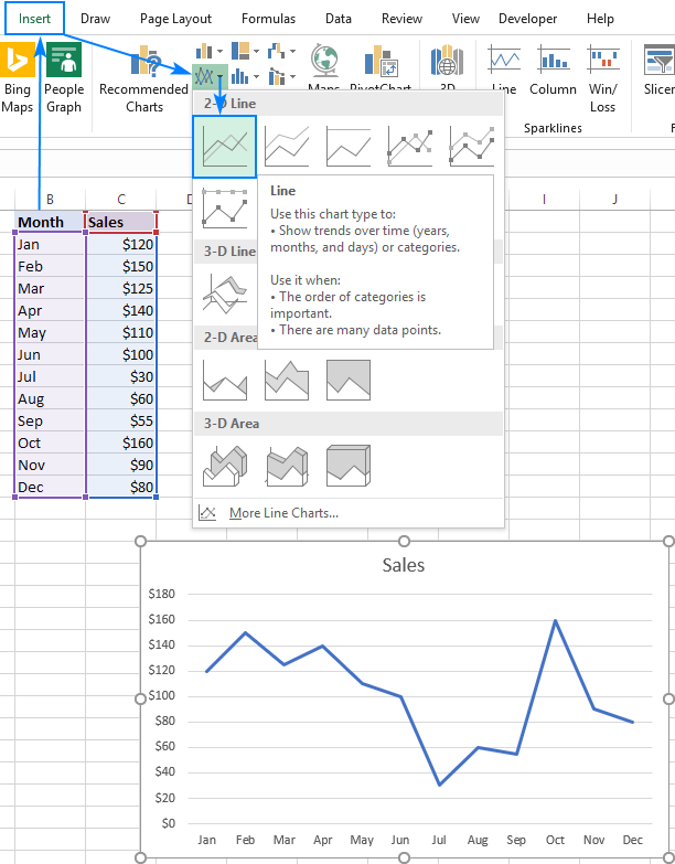
How to draw chart excel. Next, highlight the cells in the range a2:b9, then click the insert tab, then click the. Select the whole table with the. 1, how do i add a graph into excel?
Enter the data from the sample data table above. Copy the average/benchmark/target value in the new rows and leave the cells in the first two columns empty, as shown in the screenshot below. Step, 2, add a new.
Open the worksheet and click the insert button to access the my apps option. Here, we basically create an up, down, and equal trend chart. We can create a trend chart in excel using a line chart with excel shapes.
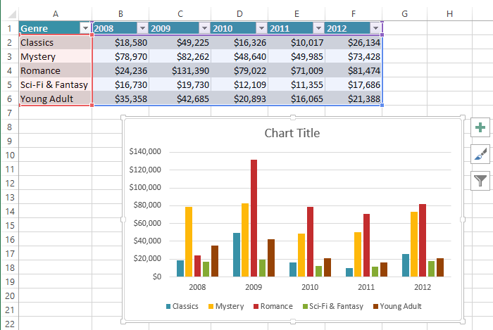
Click on smartart options under the illustrations section as per the below screenshot. How to make a graph in excel, you must select the data for which a chart is to be created. In the insert menu, select recommended charts.
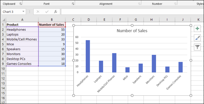
Follow the below steps to get insight. First, let’s enter the following dataset of x and y values in excel: To insert a bar chart in microsoft excel, open your excel workbook and select your data.
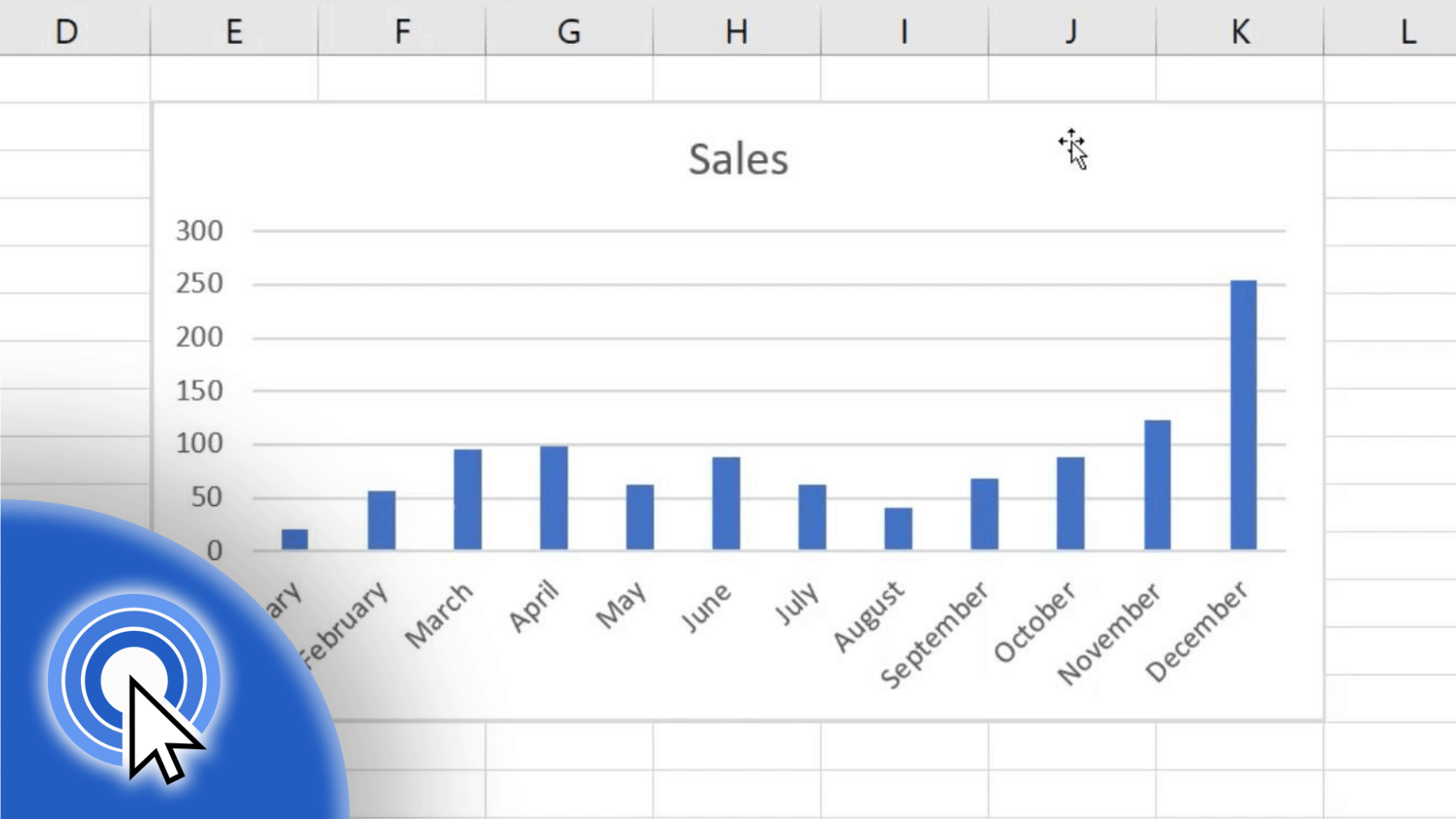
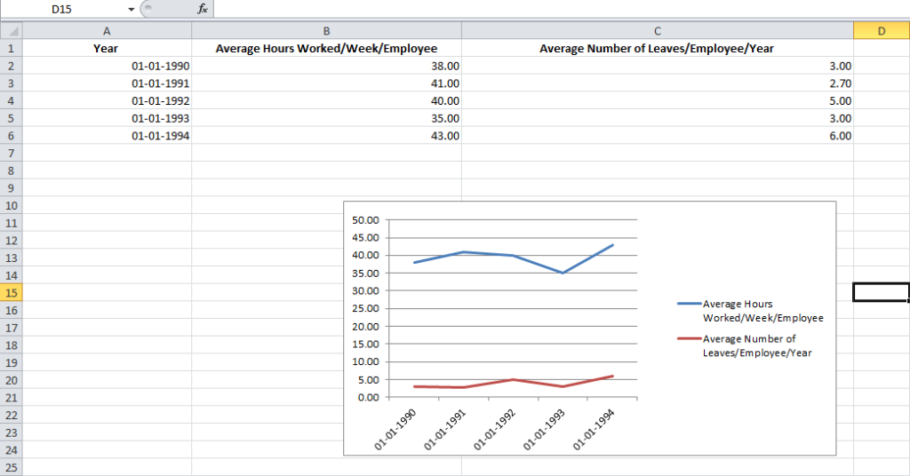
You will immediately see a graph appear below your data. To show this method, we take a dataset that. It will open a smartart graphic dialog box for various options, as shown.
This method works with all versions of excel. You can do this manually using your mouse, or you can select a cell in your range and. With the columns selected, visit the insert tab and choose the option 2d line graph.
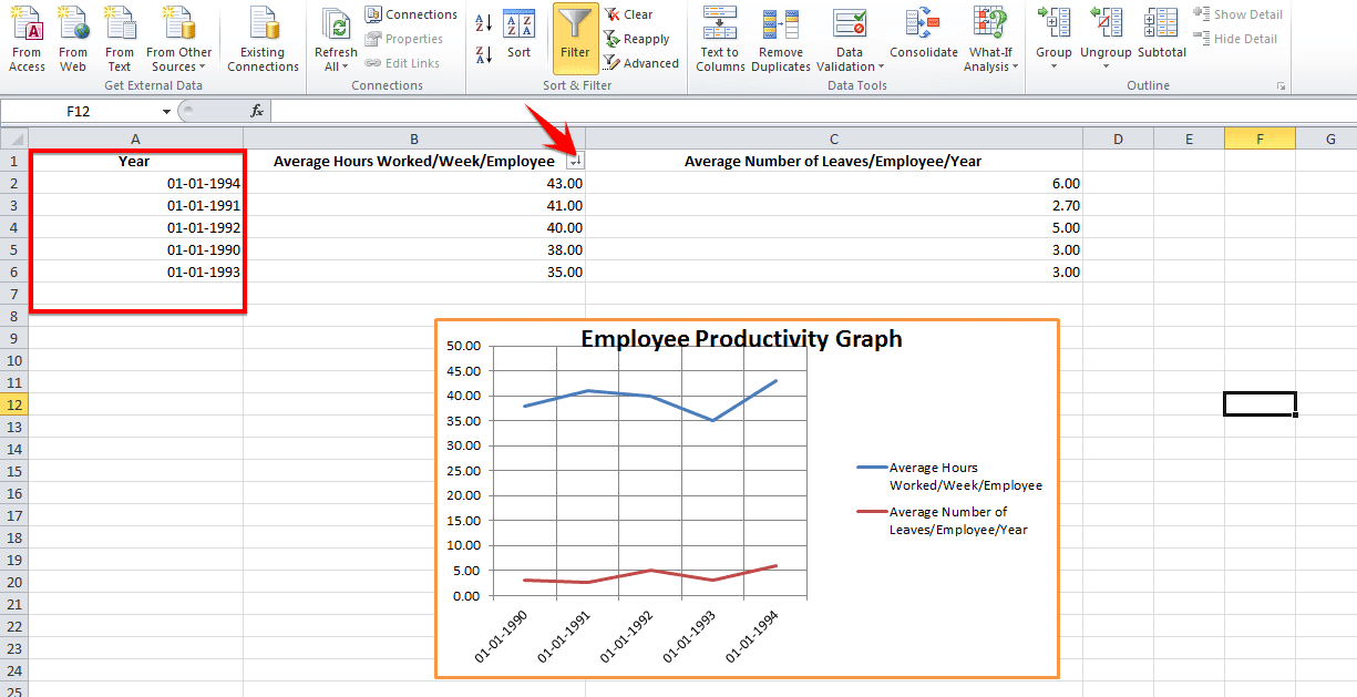
To install chartexpo into your excel, click the following link. After applying the above formula, the answer is shown below. In the cell, f1 apply the formula for “average (b2:b31)”, where the function computes the average of 30 weeks.
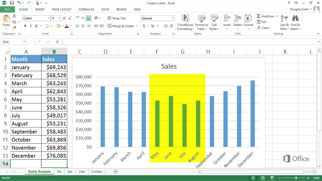
Create the basic excel graph. Choose any chart from the list of. The steps to create a waterfall chart in excel are:
Click the above table > click the “ insert ” tab > go to the “ charts ” group > click the “ insert waterfall, funnel, stock, surface, or radar. Select the data from a1 to b13. If you don't have excel 2016 or later, simply create a pareto chart by combining a column chart and a line graph.
How To Make A Chart Or Graph In Excel | Customguide
How To Make Charts And Graphs In Excel | Smartsheet
How To Make A Line Graph In Excel
How To Make A Graph In Excel: Step By Detailed Tutorial
Video: Create A Chart
Excel Quick And Simple Charts Tutorial - Youtube
Add A Data Series To Your Chart
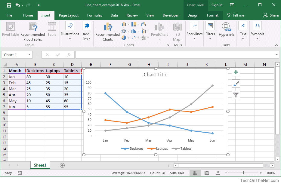
Ms Excel 2016: How To Create A Line Chart
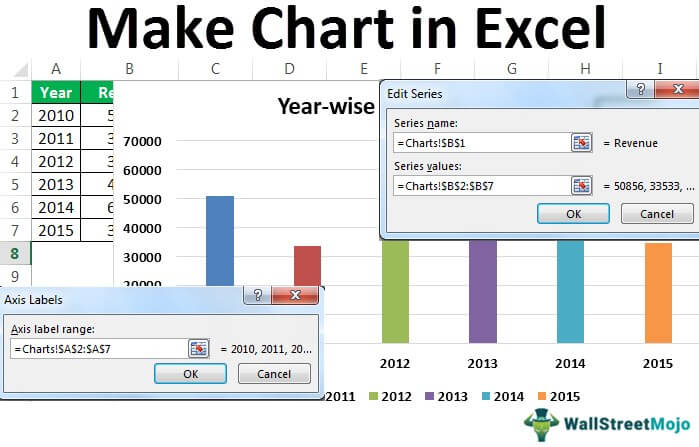
How To Make Chart Or Graph In Excel? (step By Step Examples)

How To Make A Line Graph In Excel-easy Tutorial - Youtube

How To Create A Chart By Count Of Values In Excel?
![How To Make A Chart Or Graph In Excel [With Video Tutorial]](https://lh6.googleusercontent.com/TI3l925CzYkbj73vLOAcGbLEiLyIiWd37ZYNi3FjmTC6EL7pBCd6AWYX3C0VBD-T-f0p9Px4nTzFotpRDK2US1ZYUNOZd88m1ksDXGXFFZuEtRhpMj_dFsCZSNpCYgpv0v_W26Odo0_c2de0Dvw_CQ)
How To Make A Chart Or Graph In Excel [with Video Tutorial]
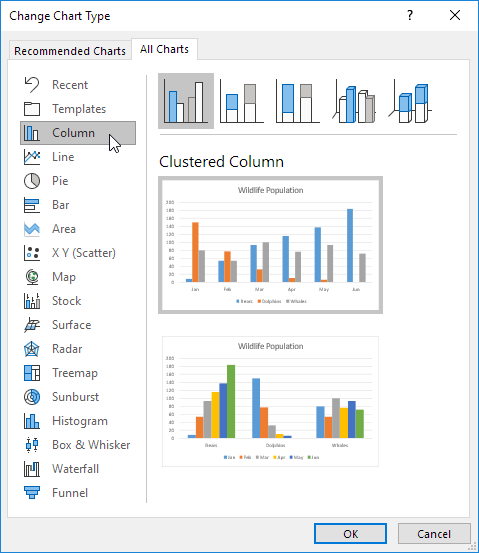
How To Create Charts In Excel (in Easy Steps)